1 PCA 在解决实际问题的时候,多变量问题是经常会遇到的,变量太多,无疑会增加分析问题的难度与复杂性。同时,在许多实际问题中,多个变量之间是具有一定的相关关系的。因此,能否在各个变量之间相关关系研究的基础上, 用较少的新变量代替原来较多的变量,而且使这些较少的新变量尽可能多地保留原来较多的变量所反映的信息?事实上,这种想法是可以实现的。
1.1 原理 PCA (Principal Components Analysis,,主成分分析)是将原来多个变量化为少数几个综合指标的一种统计分析方法,从数学角度来看,这是一种降维处理技术。 下面举例说明其原理,加入有以下数据:
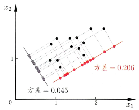
可以将上述数据看成一个椭圆形,椭圆有一个长轴和一个短轴。 在短轴方向上, 数据变化很少;在极端的情况,短轴如果退化成一点, 那只有在长轴的方向才能够解释这些点的变化了。这样,由二维到一维的降维就自然完成了。 从数据波动上来看,在短轴上数据的方差较小,因此在该轴上的信息属于次信息;而在长轴上数据的方差较大,因此在该轴上的信息属于主信息。了解 PCA 的基本原理之后,我们还要思考一个问题,PCA 优化的目标是什么?请看下图:
我们将上图中的点往两个超平面上投影,分别得到不同超平面的方差分别为:0.045,0.206,因此将所有样本点投影到方差为 0.206 的超平面能在实现降维的目标且保留更多的信息。因此 PCA 要做得是使所有样本的投影尽可能分开,也即找到一个样本投影后的方差最大的超平面来实现降维。我们将上述降维准则称作 最大可分性 ;同时样本点到这个超平面的距离都足够近,即下图中所有红线(即投影造成的损失)加起来最小,也就是保留了更多的信息,我们将此准则称作 最近重构性 。
1.2 算法流程 PCA 整体的算法流程描述如下:
输入:样本集 $\boldsymbol{D = {x_1,x_2, \cdots,x_m}}$; 低维空间维数 $\boldsymbol{k}$;
过程:
1:对所有样本进行零均值化:$\boldsymbol{x_i\leftarrow x_i - \frac{1}{m}\sum_{i=1}^{m}x_i}$;
2:计算样本的协方差矩阵 $\boldsymbol{XX^T}$;
3:对协方差矩阵 $\boldsymbol{XX^T}$ 做特征值分解;
4:取最大的 $\boldsymbol{k}$ 个的特征值所对应的特征向量 $\boldsymbol{w_1, w_2, \cdots, w_{k}}$;
输出:投影矩阵 $\boldsymbol{W = (w_1, w_2, \cdots, w_{k})}$。
下面对每个步骤进行详细分析。
1.2.1 零均值化 此步骤的目的是标准化输入数据集,使数据成比例缩小。更确切地说,在使用 PCA 之前必须标准化数据的原因是 PCA 方法对初始变量的方差非常敏感。也就是说,如果初始变量的范围之间存在较大差异,那么范围较大的变量占的比重较大,和较小的变量相比(例如,范围介于 0 和 100 之间的变量较 0 到 1 之间的变量会占较大比重),这将导致主成分的偏差。通过将数据转换为同样的比例可以防止这个问题。在实现过程中,我们的操作区别于标准的标准化,我们只将每个样本减去它们的均值。
1.2.2 计算协方差矩阵 此步骤的目的是了解输入数据集的变量相对于彼此平均值变化,换句话说,查看它们是否存在关系。因为有时候变量由于高度相关,这样就会包含冗余信息。因此,为了识别变量的相关性,我们计算协方差矩阵。下面以二维矩阵为例:
上述矩阵中,对角线上分别是特征 $x, y,z$ 的方差,非对角线上是协方差。由于协方差是可交换的 $Cov(a, b) = Cov(b,a)$,协方差矩阵关于主对角线是对称的,这意味着上三角部分和下三角部分相等。协方差矩阵可以告诉我们变量之间的关系,总结有如下三点:
如果协方差为正则:两个变量一起增加或减少(正相关);
如果协方差为负则:两个变量其中一个增加,另一个减少(负相关);
协方差绝对值越大,两者对彼此的影响越大,反之越小。
1.2.3 特征值和特征向量 求协方差矩阵 $C$ 的特征值 $\lambda$ 和相对应的特征向量 $u$ (每一个特征值对应一个特征向量):
特征值 $\lambda$ 会有 $N$ 个,每一个 $\lambda$ 对应一个特征向量 $u$,将特征值 $\lambda$ 按照从大到小的顺序排序,选择最大的前 $K$ 个,并将其相对应的 $K$ 个特征向量拿出来,我们会得到一组 $\{(\lambda_1,u_1),(\lambda_2,u_2),\cdots,(\lambda_k, u_k)\}$。为什么只取特征值较大的特征向量,因为较大特征值对应的特征向量保留了原始数据的大部分信息吗,也即方差较大,可作为数据的主成分。
1.2.4 降维得到 K 维特征 选取最大的前 $K$ 个特征值和相对应的特征向量,并进行投影的过程,就是降维的过程。对于每个样本 $X_i$,原始的特征是 $(x_1, x_2, \cdots,x_m)$,投影之后的新特征是 $(y_1,y_2,\cdots,y_k)$,计算过程如下:
1.2.5 PCA 的优缺点 优点:
只需以方差衡量信息量,不受数据集以外的因素影响;
各主成分之间正交,可消除原始数据成分间的相互影响;
计算方法简单,主要运算是特征值分解且易于实现。
缺点:
主成分各特征维度的含义具有模糊性,不如原始样本特征的解释性强;
方差小的成分可能含有影响样本差异的重要信息,降维丢弃可能对后续数据处理有影响。
2 Python 实现 PCA 本次实现的流程完全依据于 1.2 算法流程
1
2
3
4
5
6
7
8
9
10
11
12
13
14
15
16
17
18
19
20
21
22
23
24
25
26
27
28
class PCA : def __init__ (self, n_components ): self.n_components = n_components def fit (self, X ): X_mean = np.mean(X, axis = 0 ) X_norm = X - X_mean X_conv = np.cov(X_norm, rowvar = False ) eigenvalues, featurevectors = np.linalg.eig(X_conv) index = np.argsort(eigenvalues) n_index = index[ -self.n_components : ] self.w = featurevectors[ : , n_index] return self def transform (self, X ): eigenfaces = np.dot(X, self.w) return eigenfaces
3 基于 PCA 的人脸识别 在前面中,我们从原理开始分析 PCA 算法,最终并使用 Python 实现了 PCA 算法,那这部分主要是使用 PCA 来对不同的人脸识别数据集进行提取特征,并且实现人脸识别。
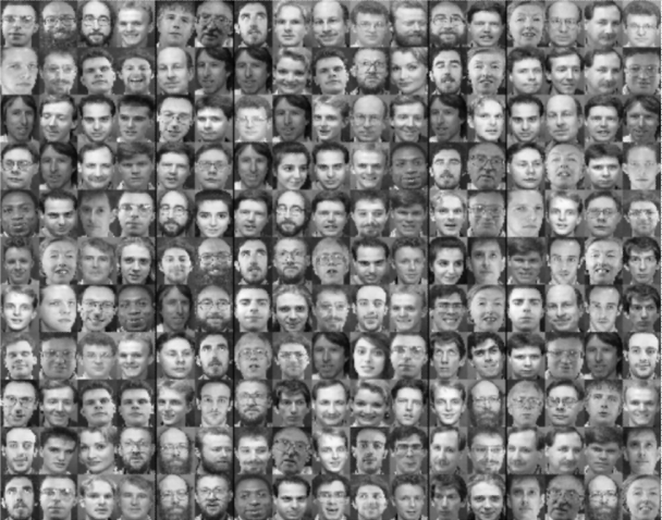
3.1 ORL 数据集 ORL 人脸数据集共包含 40 个不同人的 400 张图像,是在 1992 年 4 月至 1994 年 4 月期间由英国剑桥的 Olivetti 研究实验室创建。 此数据集下包含 40 个目录,每个目录下有 10 张图像,每个目录表示一个不同的人。所有的图像是以 PGM 格式存储,灰度图,图像大小宽度为 92,高度为 112。对每一个目录下的图像,这些图像是在不同的时间、不同的光照、不同的面部表情 (睁眼 / 闭眼,微笑 / 不微笑) 和面部细节 (戴眼镜 / 不戴眼镜) 环境下采集的。所有的图像是在较暗的均匀背景下拍摄的,拍摄的是正脸 (有些带有略微的侧偏)。下载地址为:https://github.com/yasminemedhat/Face-Recognition
人脸识别的流程如下:
数据读取与数据处理;
数据分组;
使用 PCA 进行特征提取;
人脸识别;
人脸识别的 GUI 界面。
3.1.1 数据读取与数据处理 因为 ORL 数据集的图片格式是 .pgm ,我使用了 pillow 库中的 Image 类来进行读取。对于每张照片将其拉直,因为 ORL 中图片大小是 (112,92),拉直之后则变成 (10304,),然后将所有照片进行拼接,最终得到大小为 (400,10304) 的二维矩阵。再者就是标签的构造,从上到下的 人 的标签分别是 0,1,2,…,39,要注意每一张图片都要有一个标签。
1
2
3
4
5
6
7
8
9
10
11
12
13
14
15
16
def Data_Processing (root ) : X = [] y = [] path_list = ['s' + str (i) for i in range (1 , 41 )] for idx, s in enumerate (path_list) : for i in range (1 , 11 ) : path = os.path.join(root, s, str (i) + '.pgm' ) img = Image.open (path) img = np.array(img).ravel() X.append(img) y.extend([idx] * 10 ) X = np.array(X) y = np.array(y) return X, y
3.1.2 数据分组 本次数据的分割依据于下面的两种方式:
每个人的前面 8 张照片作为训练并作为测试样本库,后面 2 张作为测试待识别图片;
前 38 个人作为训练,后 12 个人作为测试,其中测试库中每个人的前面 8 张照片为测试样本库,后面 2 张照片作为待识别图片。
1
2
3
4
5
6
7
8
9
10
11
12
13
14
15
16
17
18
19
20
21
22
23
24
25
26
27
28
29
30
31
32
33
34
35
36
37
38
def Data_Split (X, y, flag ) : train_set = [] train_target = [] test_set = [] test_target = [] face_unrecognized_set = [] face_unrecognized_target = [] if flag == 1 : for i in range (40 ) : train_set.append(X[i * 10 : i * 10 + 8 ]) train_target.extend(y[i * 10 : i * 10 + 8 ]) face_unrecognized_set.append(X[i * 10 + 8 : (i + 1 ) * 10 ]) face_unrecognized_target.extend(y[i * 10 + 8 : (i + 1 ) * 10 ]) test_set = train_set.copy() test_target = train_target.copy() else : train_set = X[: 380 , :] train_target = y[: 380 ] X_temp = X[380 :, :] y_temp = y[380 :] for i in range (2 ) : test_set.extend(X_temp[i * 10 : i * 10 + 8 ]) test_target.extend(y_temp[i * 10 : i * 10 + 8 ]) face_unrecognized_set.extend(X_temp[i * 10 + 8 : (i + 1 ) * 10 ]) face_unrecognized_target.extend(y_temp[i * 10 + 8 : (i + 1 ) * 10 ]) train_set = np.array(train_set) train_target = np.array(train_target) test_set = np.array(test_set) test_target = np.array(test_target) face_unrecognized_set = np.array(face_unrecognized_set) face_unrecognized_target = np.array(face_unrecognized_target) return train_set, train_target, \ test_set, test_target, \ face_unrecognized_set, face_unrecognized_target
3.1.3 使用 PCA 进行特征提取 本过程对人脸特征进行提取,主要难度在于编写 PCA,我们在前面已经完成。但是我们还有一个非常重要的参数要确定,就是 $\boldsymbol{k}$ 值,如果 $\boldsymbol{k}$ 过大,那 PCA 降维之后数据信息中仍然保留大量的冗余信息;如果 $\boldsymbol{k}$ 过小,则 PCA 降维过程中损失了过多信息,不利于后续的识别工作。为此,我借用 sklearn 来探究在保留 95% 的原始数据应该降到多少纬合适。
1
2
3
4
from sklearn.decomposition import PCApca = PCA(n_components = 0.95 ) pca.fit(train_set) print (pca.n_components_)
最终的测试结果是对于 分组一 和 分组二 的 $\boldsymbol{k}$ 值分别是 161,184。知道 $\boldsymbol{k}$ 值之后,我们就可以进行特征提取,要注意我们只能对训练集进行训练,也即要使用训练集的特征向量对测试集和待识别图片进行 PCA 降维。
1
2
3
4
5
pca = PCA(n_components = 161 ) pca.fit(train_set) train_reduction = pca.transform(train_set) test_reduction = pca.transform(test_set) face_unrecognized_reduction = pca.transform(face_unrecognized_set)
3.1.4 人脸识别 经过上述步骤之后,我们可以得到降维后的训练集、测试集和待识别人脸,在这部分我们就可以进行人脸匹配。首先要说明:对于人脸识别而言,如果计算机先前没有看到过关于这个人的照片,那对这个人进行人脸识别是没有意义的,大家可以细细探究一下 分组一 和 分组二 。本次人脸识别我使用的准则是 二范数 ,下面分别对 分组一 和 分组二 进行讲解。
首先是 分组一 ,因为训练集和测试集一样,都包含了全部人的人脸,也就是说计算机 “看过” 待识别人脸,因此我们可以用训练集或者测试集来进行人脸识别:计算待识别的人脸特征向量与训练集中每一张图片的特征向量的二范数,其中二范数最小的那张图片就是我们在训练集中匹配到的人脸。在此过程我设置了两个返回值分别是 pred 和 labels ,前者为匹配到的人脸图片在训练集中的下标,方便后面的 GUI 设计,后者是匹配到的人脸图片的标签,用于后续的识别准确率。
1
2
3
4
5
6
7
8
9
def Predict (X, Y ) : labels = [] pred = [] for i in range (len (Y)) : distance = np.linalg.norm(X - Y[i], axis = 1 ) label = np.argmin(distance) labels.append(label // 8 ) pred.append(label) return np.array(labels), np.array(pred)
其次是 分组二 ,训练集是前 38 个人的人脸照片,测试集是后两个人的前 8 张图片,待识别图片是后两个人的后两张人脸图片。如果我们使用训练集去匹配待识别图片,这时计算原先没有 “看过” 该人人脸,此时识别是无意义的,因此我们要使用测试集去识别待识别图片。返回值同样是 pred 和 labels ,要注意标签的计算方式。
1
2
3
4
5
6
7
8
9
def Predict (X, Y ) : labels = [] pred = [] for i in range (len (Y)) : distance = np.linalg.norm(X - Y[i], axis = 1 ) label = np.argmin(distance) labels.append(label // 8 + 38 ) pred.append(label) return np.array(labels), np.array(pred)
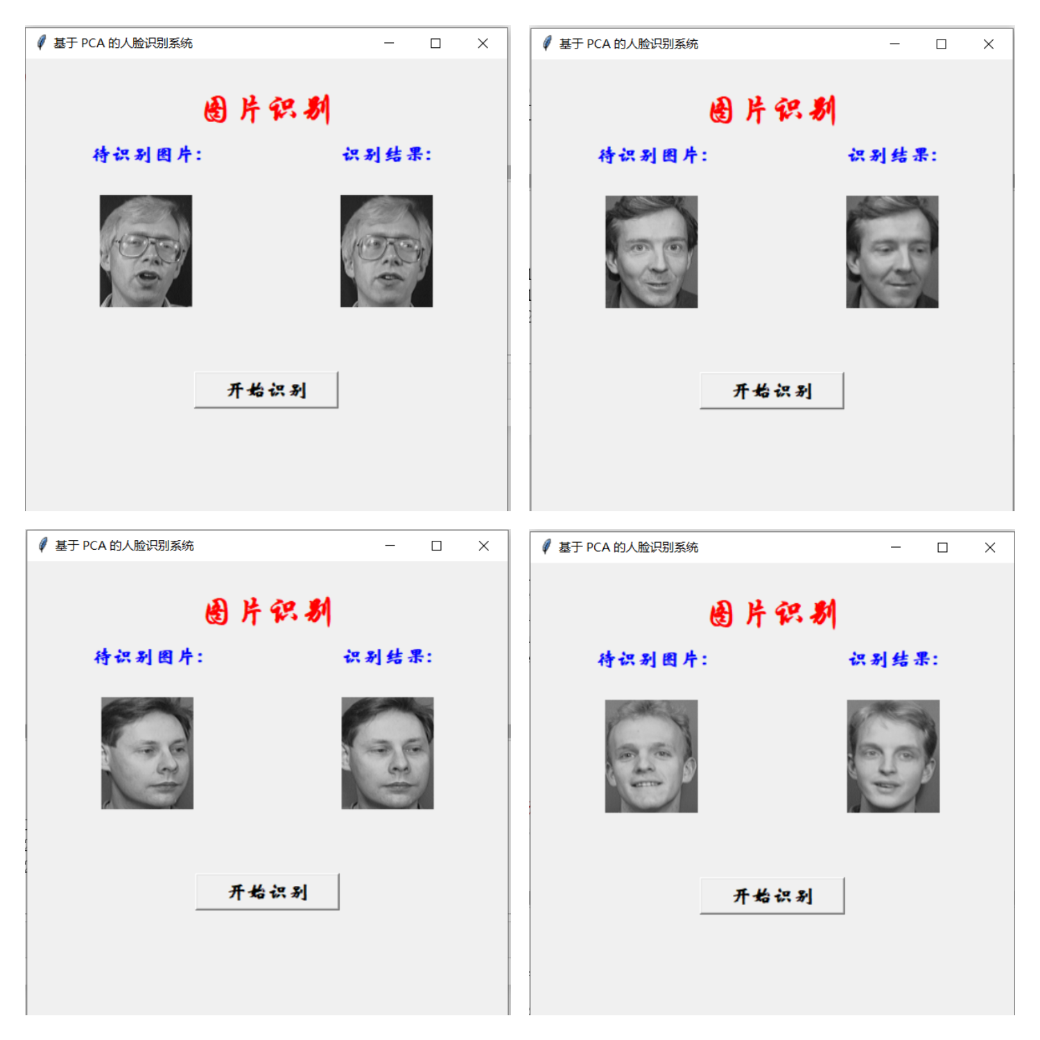
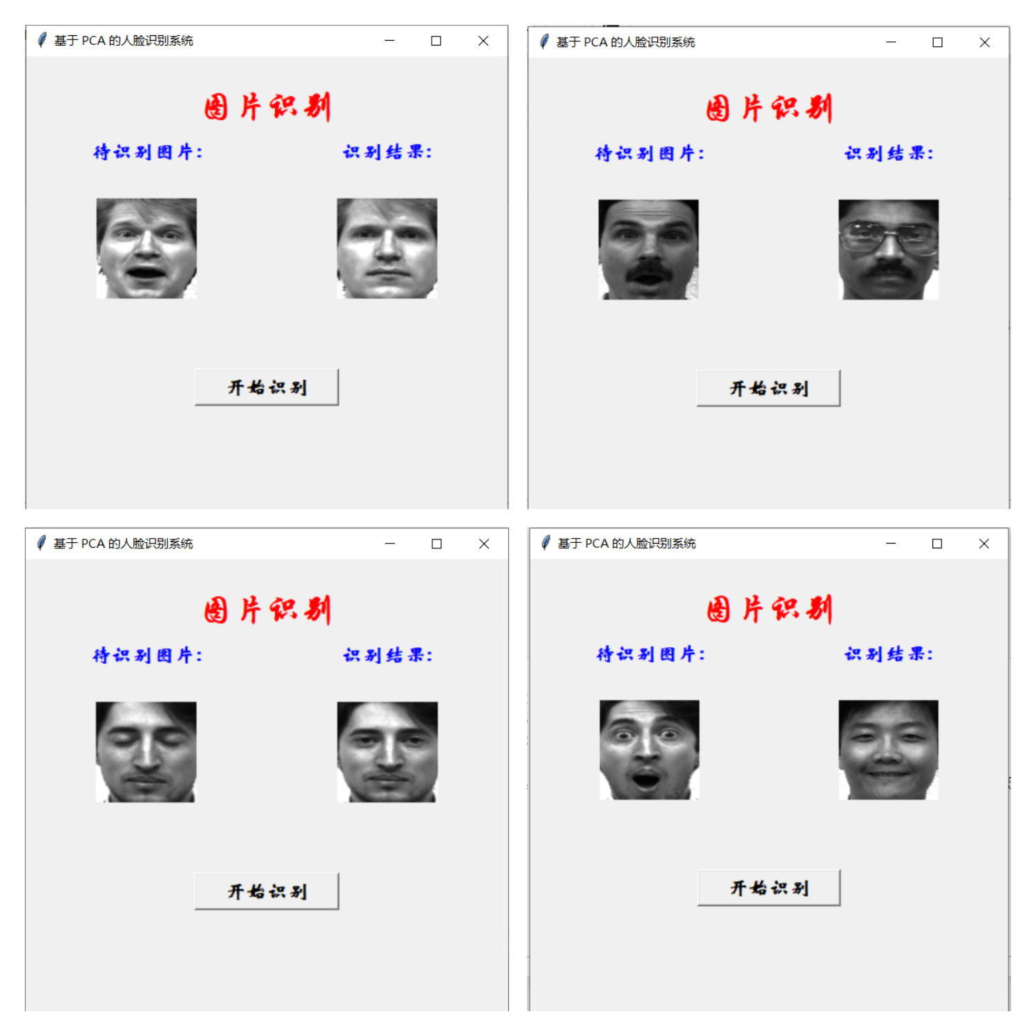
3.1.5 人脸识别的 GUI 界面 为了体现人脸识别系统的完整性,我设计了人脸识别系统的 GUI,在 GUI 页面的左边展示的是待识别人脸图片,在点击按键 “开始识别” 之后,GUI 页面右边会展示识别效果。代码与效果会在下面展示。
3.1.6 实验结果 对于分组一:一共有采集了 80 张待识别人脸图片,最终识别正确率是 0.95,显示别效果如下:
如上图,前面三张识别是成功的,而第四张是识别错误的。
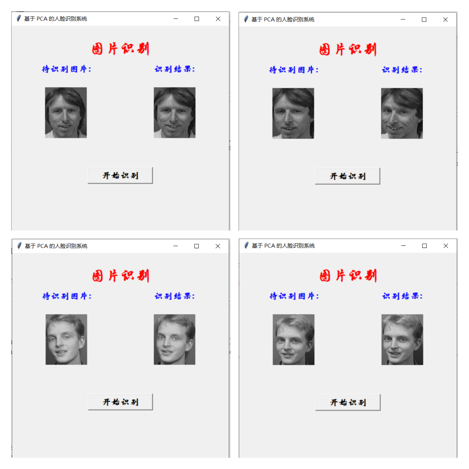
对于分组二:一共有采集了 4 张待识别人脸图片,最终识别正确率是 1.0,显示别效果如下:
如上图,四张待识别图片全部识别正确。
3.1.7 全部代码 1 2 3 4 5 6 7 8 9 10 11 12 13 14 15 16 17 18 19 20 21 22 23 24 25 26 27 28 29 30 31 32 33 34 35 36 37 38 39 40 41 42 43 44 45 46 47 48 49 50 51 52 53 54 55 56 57 58 59 60 61 62 63 64 65 66 67 68 69 70 71 72 73 74 75 76 77 78 79 80 81 82 83 84 85 86 87 88 89 90 91 92 93 94 95 96 97 98 99 100 101 102 103 104 105 106 107 108 109 110 111 112 113 114 115 116 117 118 119 120 121 122 123 124 125 126 127 128 129 130 131 132 133 134 135 136 137 138 139 140 141 142 143 144 145 146 147 148 149 150 151 152 153 154 155 156 import numpy as npimport osfrom tkinter import *from PIL import Image, ImageTkfrom tkinter import fontclass PCA : def __init__ (self, n_components ): self.n_components = n_components def fit (self, X ): X_mean = np.mean(X, axis = 0 ) X_norm = X - X_mean X_conv = np.cov(X_norm, rowvar = False ) eigenvalues, featurevectors = np.linalg.eig(X_conv) index = np.argsort(eigenvalues) n_index = index[ -self.n_components : ] self.w = featurevectors[ : , n_index] return self def transform (self, X ): eigenfaces = np.dot(X, self.w) return eigenfaces def Data_Processing (root ) : X = [] y = [] path_list = ['s' + str (i) for i in range (1 , 41 )] for idx, s in enumerate (path_list) : for i in range (1 , 11 ) : path = os.path.join(root, s, str (i) + '.pgm' ) img = Image.open (path) img = np.array(img).ravel() X.append(img) y.extend([idx] * 10 ) X = np.array(X) y = np.array(y) return X, y def Data_Split (X, y, flag ) : train_set = [] train_target = [] test_set = [] test_target = [] face_unrecognized_set = [] face_unrecognized_target = [] if flag == 1 : for i in range (40 ) : train_set.append(X[i * 10 : i * 10 + 8 ]) train_target.extend(y[i * 10 : i * 10 + 8 ]) face_unrecognized_set.append(X[i * 10 + 8 : (i + 1 ) * 10 ]) face_unrecognized_target.extend(y[i * 10 + 8 : (i + 1 ) * 10 ]) test_set = train_set.copy() test_target = train_target.copy() else : train_set = X[: 380 , :] train_target = y[: 380 ] X_temp = X[380 :, :] y_temp = y[380 :] for i in range (2 ) : test_set.extend(X_temp[i * 10 : i * 10 + 8 ]) test_target.extend(y_temp[i * 10 : i * 10 + 8 ]) face_unrecognized_set.extend(X_temp[i * 10 + 8 : (i + 1 ) * 10 ]) face_unrecognized_target.extend(y_temp[i * 10 + 8 : (i + 1 ) * 10 ]) train_set = np.array(train_set) train_target = np.array(train_target) test_set = np.array(test_set) test_target = np.array(test_target) face_unrecognized_set = np.array(face_unrecognized_set) face_unrecognized_target = np.array(face_unrecognized_target) return train_set, train_target, \ test_set, test_target, \ face_unrecognized_set, face_unrecognized_target def Predict (X, Y ) : labels = [] pred = [] for i in range (len (Y)) : distance = np.linalg.norm(X - Y[i], axis = 1 ) label = np.argmin(distance) labels.append(label // 8 ) pred.append(label) return np.array(labels), np.array(pred) def Face_GUI (unrecognized, result ) : img = unrecognized.reshape(112 , 92 ) img = Image.fromarray(img) photo = ImageTk.PhotoImage(img) label = Label(root, text = "图片识别" , fg = 'red' , font = ("华文行楷" , 25 , font.BOLD)) label.place(relx = 0.35 , rely = 0.01 , relwidth = 0.3 , relheight = 0.2 ) lb1 = Label(root, image = photo) lb1.place(relx = 0.1 , rely = 0.25 , relwidth = 0.3 , relheight = 0.3 ) label_context1 = Label(root, text = "待识别图片:" , fg = 'blue' , font = ("华文新魏" , 15 , font.BOLD)) label_context1.place(relx = 0.1 , rely = 0.15 , relwidth = 0.3 , relheight = 0.1 ) btn = Button(root, text = "开始识别" , command = lambda : Match(result), font = ("华文新魏" , 15 , font.BOLD)) btn.place(relx = 0.35 , rely = 0.65 , relwidth = 0.3 ) root.mainloop() def Match (result ) : img = result.reshape(112 , 92 ) img = Image.fromarray(img) photo = ImageTk.PhotoImage(img) lb2 = Label(root, image = photo) lb2.place(relx = 0.6 , rely = 0.25 , relwidth = 0.3 , relheight = 0.3 ) label_context2 = Label(root, text = "识别结果:" , fg = 'blue' , font = ("华文新魏" , 15 , font.BOLD)) label_context2.place(relx = 0.6 , rely = 0.15 , relwidth = 0.3 , relheight = 0.1 ) root.mainloop() if __name__ == '__main__' : X, y = Data_Processing('ORL' ) train_set, train_target, test_set, test_target, face_unrecognized_set,\ face_unrecognized_target = Data_Split(X, y, flag = 1 ) pca = PCA(n_components = 161 ) pca.fit(train_set) train_reduction = pca.transform(train_set) test_reduction = pca.transform(test_set) face_unrecognized_reduction = pca.transform(face_unrecognized_set) labels, pred = Predict(train_reduction, face_unrecognized_reduction) accuracy = (labels == face_unrecognized_target).sum () / len (face_unrecognized_target) print (accuracy) print (pred) for i in range (len (pred)): root = Tk() root.geometry('480x480' ) root.title('基于 PCA 的人脸识别系统' ) unrecognized = face_unrecognized_set[i] result = train_set[pred[i]] Face_GUI(unrecognized, result)
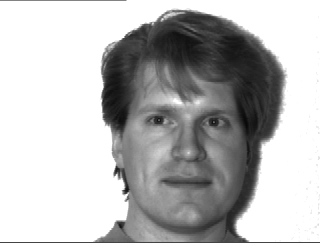
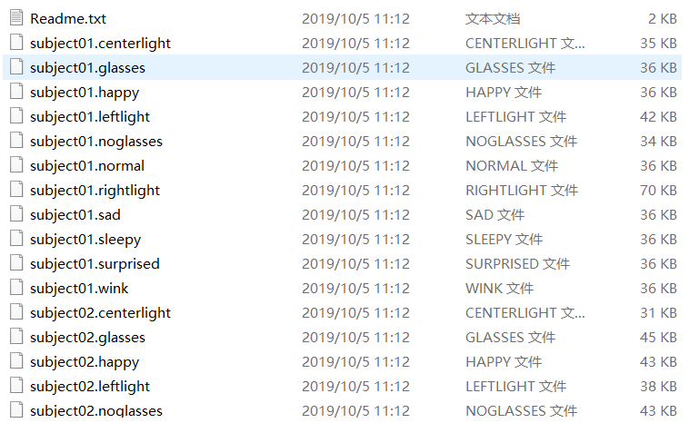
3.2 Yale 数据集 Yale 人脸数据库是一个人脸数据集,主要用于身份鉴定,包含 15 个人,其中每个人有 11 张图像共计 165 个 GIF 格式的灰度图像,每个主题包含不同的面部表情:中心光、带眼镜、快乐、左光、没有眼镜、正常、右光、悲伤、困、惊讶和眨眼。图像大小宽度为 320,高度为 243。下载地址为:https://www.kaggle.com/datasets/olgabelitskaya/yale-face-database
使用 PCA 对 Yale数据集进行人脸识别的流程和对 ORL 数据集的流程一样,但是许多细节需要调整。
3.2.1 数据读取和数据处理 Yale 数据集的文件形式不是我们常见的图片编码格式,因此我使用了 skimage 包中的 io 模块对图片进行读取。
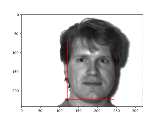
在读取完之后,我们发现原始的人脸图片很大,其大小为我们前面所讲的 (243,320),一张图中,背景占比很高,如果直接对原图进行展平得到 (77760,) 大小的向量,这对于计算资源的要求很高,而且因为背景的存在会影响人脸特征的提取,并最终影响人脸识别性能。因此,一般的人脸识别系统在特征提取之前会首先做一件事:人脸检测 。不能此实验我使用热人脸检测模型是 MTCNN 这是一个深度学习模型,可以达到实施效果,且准确率非常高。可以在命令行通过以下命令进行安装:
MTCNN 的使用模板如下:
1
2
3
4
from mtcnn.mtcnn import MTCNNdetector = MTCNN() result = detector.detect_faces(img)
返回值为:要注意的是返回的结果可能有多个人脸。
1 2 3 4 5 6 7 [{'box ': [121 , 69 , 122 , 154 ], 'confidence ': 0.9999041557312012 , 'keypoints ': {'left_eye ': (160 , 122 ), 'right_eye ': (214 , 123 ), 'nose ': (189 , 152 ), 'mouth_left ': (163 , 182 ), 'mouth_right ': (210 , 184 )}}]
关于 MTCNN 可以参考:https://arxiv.org/abs/1604.02878
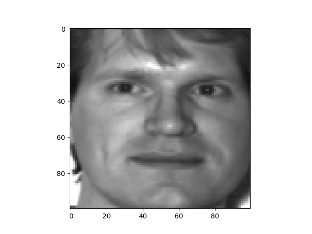
在人脸检测之后,就可以根据结果中的人脸框信息对原图的人脸区域进行裁剪,同时为保证最后提取特征的图片向量维度一致,将裁取图片进行 resize 到 (100,100)。
得到人脸区域之后,我们将该区域展平成向量,以便后续操作。
1
2
3
4
5
6
7
8
9
10
11
12
13
14
15
16
17
18
19
20
21
22
23
24
25
26
27
28
29
30
31
32
33
34
35
36
37
38
39
40
41
42
43
44
45
46
47
48
49
50
51
52
53
def Draw_image_with_boxes (data, result_list ): plt.imshow(data) ax = plt.gca() for result in result_list: print (result) x, y, width, height = result['box' ] rect = Rectangle((x, y), width, height, fill = False , color = 'red' ) ax.add_patch(rect) plt.show() def Data_Processing (root ) : Yale_path = [] X = [] y = [] faces = [] for element in os.listdir(root) : if element != 'Readme.txt' : Yale_path.append(os.path.join(root, element)) for path in Yale_path : image = io.imread(path, as_gray = True ) X.append(image) label = int (os.path.split(path)[-1 ].split('.' )[0 ].replace("subject" , "" )) - 1 y.append(label) detector = MTCNN() for img_src in X : img = np.stack((img_src, img_src, img_src), axis = 2 ) result = detector.detect_faces(img) box = result[0 ]['box' ] img1 = img_src[box[1 ] : box[1 ] + box[3 ], box[0 ] : box[0 ] + box[2 ]] image = Image.fromarray(img1) image = image.resize((100 , 100 )) face_array = np.asarray(image) faces.append(face_array.ravel()) faces = np.array(faces) y = np.array(y) print (faces.shape) return faces, y
3.2.2 数据分组 对于 Yale 数据集,我没有像 ORL 数据集那样分组,我直接取每个人的前 8 张图片作为预测集,取每个人的后 3 张图片作为待识别图片,也即训练集维度为 (120,10000),待识别图片为 (45,10000)。
1
2
3
4
5
6
7
8
9
10
11
12
13
14
15
16
17
18
def Data_Split (X, y ) : train_set = [] train_target = [] face_unrecognized_set = [] face_unrecognized_target = [] for i in range (15 ) : train_set.extend(X[i * 11 : i * 11 + 8 ]) train_target.extend(y[i * 11 : i * 11 + 8 ]) face_unrecognized_set.extend(X[i * 11 + 8 : (i + 1 ) * 11 ]) face_unrecognized_target.extend(y[i * 11 + 8 : (i + 1 ) * 11 ]) train_set = np.array(train_set) train_target = np.array(train_target) face_unrecognized_set = np.array(face_unrecognized_set) face_unrecognized_target = np.array(face_unrecognized_target) return train_set, train_target, \ face_unrecognized_set, face_unrecognized_target
3.2.3 使用 PCA 进行特征提取 我们在 3.1.3 使用 PCA 进行特征提取
1
2
3
4
pca = PCA(n_components = 46 ) pca.fit(train_set) train_reduction = pca.transform(train_set) face_unrecognized_reduction = pca.transform(face_unrecognized_set)
3.2.4 人脸识别及可视化 Yale 数据集的标签预测过程与 ORL 数据集的分组一一样,且人脸识别的 GUI 界面也与前面一样。3.1.4 人脸识别 3.1.5 人脸识别的 GUI 界面
1 img = result.reshape(100 , 100 )
3.2.5 实验结果 基于 PCA 算法构建的人脸识别系统对 Yale 数据集的识别正确率有 0.933,这是一个非常不错的正确率,因为 Yale 数据集的外界扰动十分大。识别效果如下:
如上图,一些光照变换很大、戴眼镜的人脸都能识别成,在右下角是一张识别错误的人脸,跟 ORL 数据集相比,PCA 对 Yale 数据集的鲁棒性会稍差一点。
3.2.6 全部代码 1 2 3 4 5 6 7 8 9 10 11 12 13 14 15 16 17 18 19 20 21 22 23 24 25 26 27 28 29 30 31 32 33 34 35 36 37 38 39 40 41 42 43 44 45 46 47 48 49 50 51 52 53 54 55 56 57 58 59 60 61 62 63 64 65 66 67 68 69 70 71 72 73 74 75 76 77 78 79 80 81 82 83 84 85 86 87 88 89 90 91 92 93 94 95 96 97 98 99 100 101 102 103 104 105 106 107 108 109 110 111 112 113 114 115 116 117 118 119 120 121 122 123 124 125 126 127 128 129 130 131 132 133 134 135 136 137 138 139 140 141 142 143 144 145 146 147 148 import osimport numpy as npimport matplotlib.pyplot as pltfrom PCA import PCAfrom tkinter import *from PIL import Image, ImageTkfrom tkinter import fontfrom skimage import iofrom mtcnn.mtcnn import MTCNNfrom matplotlib.patches import Rectangledef Draw_image_with_boxes (data, result_list ): plt.imshow(data) ax = plt.gca() for result in result_list: print (result) x, y, width, height = result['box' ] rect = Rectangle((x, y), width, height, fill = False , color = 'red' ) ax.add_patch(rect) plt.show() def Data_Processing (root ) : Yale_path = [] X = [] y = [] faces = [] for element in os.listdir(root) : if element != 'Readme.txt' : Yale_path.append(os.path.join(root, element)) for path in Yale_path : image = io.imread(path, as_gray = True ) X.append(image) label = int (os.path.split(path)[-1 ].split('.' )[0 ].replace("subject" , "" )) - 1 y.append(label) detector = MTCNN() for img_src in X : img = np.stack((img_src, img_src, img_src), axis = 2 ) result = detector.detect_faces(img) box = result[0 ]['box' ] img1 = img_src[box[1 ] : box[1 ] + box[3 ], box[0 ] : box[0 ] + box[2 ]] image = Image.fromarray(img1) image = image.resize((100 , 100 )) face_array = np.asarray(image) faces.append(face_array.ravel()) faces = np.array(faces) y = np.array(y) print (faces.shape) return faces, y def Data_Split (X, y ) : train_set = [] train_target = [] face_unrecognized_set = [] face_unrecognized_target = [] for i in range (15 ) : train_set.extend(X[i * 11 : i * 11 + 8 ]) train_target.extend(y[i * 11 : i * 11 + 8 ]) face_unrecognized_set.extend(X[i * 11 + 8 : (i + 1 ) * 11 ]) face_unrecognized_target.extend(y[i * 11 + 8 : (i + 1 ) * 11 ]) train_set = np.array(train_set) train_target = np.array(train_target) face_unrecognized_set = np.array(face_unrecognized_set) face_unrecognized_target = np.array(face_unrecognized_target) return train_set, train_target, \ face_unrecognized_set, face_unrecognized_target def Predict (X, Y ) : labels = [] pred = [] for i in range (len (Y)) : distance = np.linalg.norm(X - Y[i], axis = 1 ) label = np.argmin(distance) labels.append(label // 8 ) pred.append(label) return np.array(labels), np.array(pred) def Face_GUI (unrecognized, result ) : img = unrecognized.reshape(100 , 100 ) img = Image.fromarray(img) photo = ImageTk.PhotoImage(img) label = Label(root, text = "图片识别" , fg = 'red' , font = ("华文行楷" , 25 , font.BOLD)) label.place(relx = 0.35 , rely = 0.01 , relwidth = 0.3 , relheight=0.2 ) lb1 = Label(root, image = photo) lb1.place(relx = 0.1 , rely = 0.25 , relwidth = 0.3 , relheight = 0.3 ) label_context1 = Label(root, text = "待识别图片:" , fg = 'blue' , font = ("华文新魏" , 15 , font.BOLD)) label_context1.place(relx = 0.1 , rely = 0.15 , relwidth = 0.3 , relheight = 0.1 ) btn = Button(root, text = "开始识别" , command = lambda : Match(result), font = ("华文新魏" , 15 , font.BOLD)) btn.place(relx = 0.35 , rely = 0.65 , relwidth = 0.3 ) root.mainloop() def Match (result ) : img = result.reshape(100 , 100 ) img = Image.fromarray(img) photo = ImageTk.PhotoImage(img) lb2 = Label(root, image = photo) lb2.place(relx = 0.6 , rely = 0.25 , relwidth = 0.3 , relheight = 0.3 ) label_context2 = Label(root, text = "识别结果:" , fg = 'blue' , font = ("华文新魏" , 15 , font.BOLD)) label_context2.place(relx = 0.6 , rely = 0.15 , relwidth = 0.3 , relheight = 0.1 ) root.mainloop() if __name__ == '__main__' : X, y = Data_Processing('Yale' ) train_set, train_target, face_unrecognized_set, \ face_unrecognized_target = Data_Split(X, y) pca = PCA(n_components = 46 ) pca.fit(train_set) train_reduction = pca.transform(train_set) face_unrecognized_reduction = pca.transform(face_unrecognized_set) labels, pred = Predict(train_reduction, face_unrecognized_reduction) accuracy = (labels == face_unrecognized_target).sum () / len (face_unrecognized_target) print (accuracy) print (pred) for i in range (len (pred)): root = Tk() root.geometry('480x480' ) root.title('基于 PCA 的人脸识别系统' ) unrecognized = face_unrecognized_set[i] result = train_set[pred[i]] Face_GUI(unrecognized, result)
3.3 UMIST 数据集 我这里的数据集是 Sheffield 数据集,是 UMIST 数据集的 “升级版” (也就是加了几张图片),后面均以 UMIST 数据集代称。UMIST 人脸数据库由 20 个人(混合种族 / 性别 / 外貌)的 564 张图像组成(Sheffield 数据集为 575)。 每个人都显示在从侧面到正面视图的一系列姿势,每个人都在一个单独的目录中,标记为 1a、1b、…… 1t,并且图像在拍摄时连续编号。 这些文件都是 PGM 格式,大约 220 x 220 像素,256 位灰度。UMIST 数据集有两个版本,一个是原始图片,一个裁剪掉了一些背景区域,裁剪后地图片大小为 (112,92),与 ORL 数据集一样大小。为实验方便,我所用的版本是裁剪过后的版本。下载地址为:http://eprints.lincoln.ac.uk/id/eprint/16081/
未裁剪的图像示例:
裁剪图像示例:
说一个小插曲:我原本也就是想找 UMIST 数据集来做实验的,但我从前一天的晚上找到第二天早上都没找到,找到的都是一些处理好的文本数据,便放弃不找了。于是想着找 Bern 数据集来替代,却在找 Bern 数据集过程中阴差阳错地找到了 UMIST 数据集。果真我与你有缘!
3.3.1 数据读取与数据处理 对 UMIST 数据集的读取方式与 ORL 数据集有些许差别,但是处理过程与其一样,返回 3.1.1 数据读取与数据处理
1
2
3
4
5
6
7
8
9
10
11
12
13
14
15
16
17
def Data_Processing (root ) : X = [] y = [] path_files = os.listdir(root) for idx, path_file in enumerate (path_files) : path_images = os.listdir(os.path.join(root, path_file, 'face' )) for path_image in path_images : path = os.path.join(root, path_file, 'face' , path_image) img = Image.open (path) img = np.array(img) X.append(img.ravel()) y.append(idx) X = np.array(X) y = np.array(y) return X, y
3.3.2 数据分组 对于 UMIST 数据集,我取每个人的前 5 张图片作为待识别图片,每个人的其余图片为作为训练集。UMIST 数据集与 ORL、Yale 数据集都不一样,因为它每个的图片数量不一样,意味着不能按照常规方法去分割数据。这里我维护了一个 index 列表,里面存的是每个人的第一张图片的下标,index 列表从第二个元素开始每一个元素减 1 即可得到前面那个人的最后一张图片的下标。然后依据 index 列表对数据进行裁剪,最终得到的待识别图片的维度是 (100,10304),训练集图片为 (475,10304)。
1
2
3
4
5
6
7
8
9
10
11
12
13
14
15
16
17
18
19
20
21
22
23
24
25
26
def Data_Split (X, y ) : train_set = [] train_target = [] face_unrecognized_set = [] face_unrecognized_target = [] index = [] index.append(0 ) for idx in range (1 , len (y)) : if y[idx] != y[idx - 1 ] : index.append(idx) index.append(len (y)) for i in range (len (index) - 1 ) : face_unrecognized_set.extend(X[index[i] : index[i] + 5 ]) face_unrecognized_target.extend(y[index[i]: index[i] + 5 ]) train_set.extend(X[index[i] + 5 : index[i + 1 ]]) train_target.extend(y[index[i] + 5 : index[i + 1 ]]) train_set = np.array(train_set) train_target = np.array(train_target) face_unrecognized_set = np.array(face_unrecognized_set) face_unrecognized_target = np.array(face_unrecognized_target) return train_set, train_target, \ face_unrecognized_set, face_unrecognized_target
3.3.3 使用 PCA 进行特征提取 同样,我采取与前面相同的方法确定了保留原始数据 95% 信息的 $\boldsymbol{k}$ 值为 97。
1
2
3
4
5
pca = PCA(n_components = 97 ) pca.fit(train_set) train_reduction = pca.transform(train_set) face_unrecognized_reduction = pca.transform(face_unrecognized_set) labels, pred = Predict(train_reduction, face_unrecognized_reduction)
3.3.4 人脸识别及可视化 对于 UMIST 数据集,人脸识别和数据分组一样,都有一个问题就是每个人的照片数量不一样,因此在预测标签时不能简单地进行整除等操作。借鉴数据分组时的思想,我同样维护了一个 index 列表,里面存的是训练集中的每个人的第一张图片的下标,index 列表从第二个元素开始每一个元素减 1 即可得到前面那个人的最后一张图片的下标。在得到预测下标之后,用其与 index 中的元素相比较便可确定标签,更详细地比较方法参考代码如下:
1
2
3
4
5
6
7
8
9
10
11
12
13
14
15
16
17
18
19
20
def Predict (X, y, Y ): labels = [] pred = [] index = [] index.append(0 ) for idx in range (1 , len (y)): if y[idx] != y[idx - 1 ]: index.append(idx) index.append(len (y)) for i in range (len (Y)): distance = np.linalg.norm(X - Y[i], axis=1 ) label = np.argmin(distance) for j in range (len (index) - 1 ): if label >= index[j] and label < index[j + 1 ]: labels.append(j) pred.append(label) return np.array(labels), np.array(pred)
其次就是人脸识别的 GUI 页面,UMIST 数据集的 GUI 过程与 ORL 数据集一模一样,请参考前面的代码。
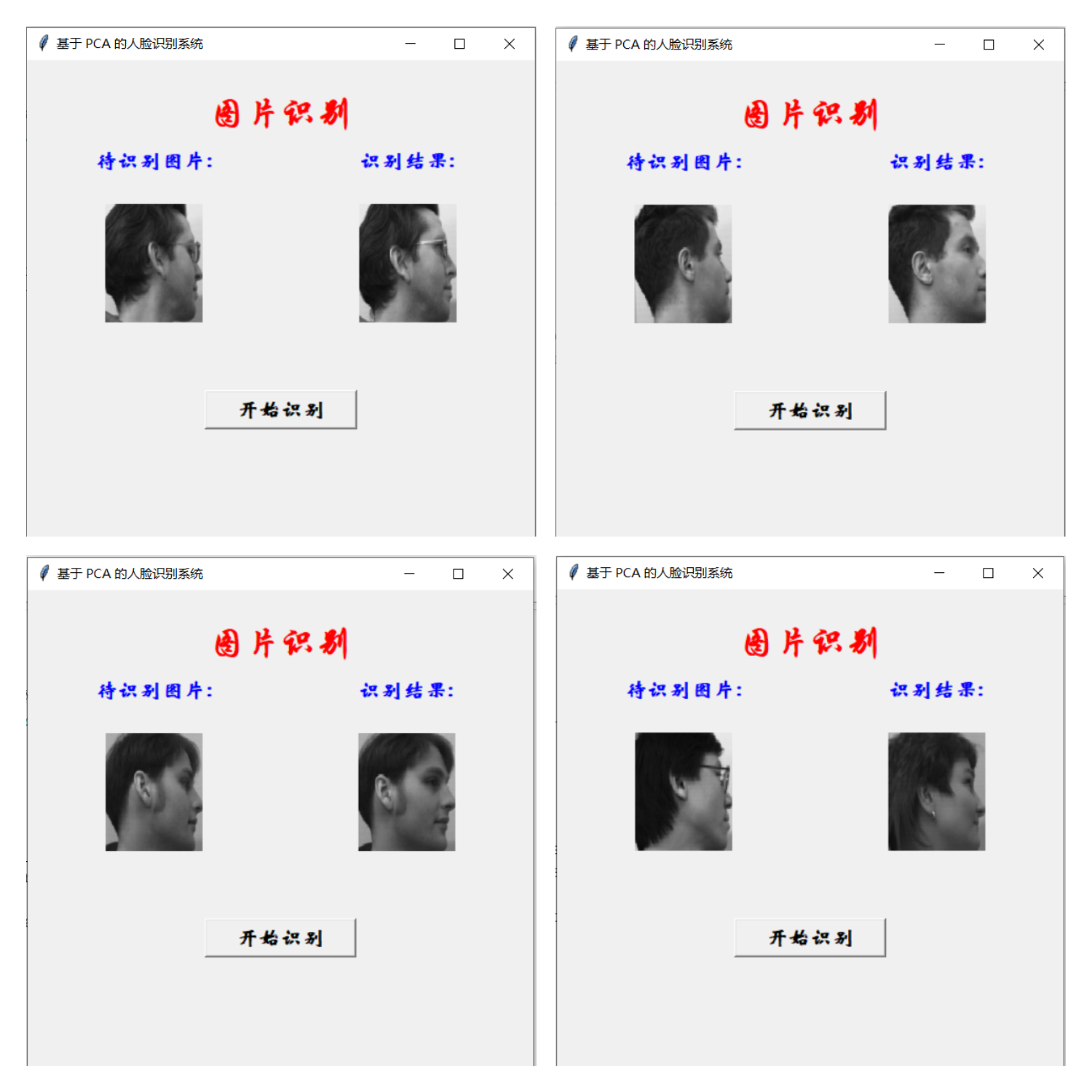
3.3.5 实验结果 基于 PCA 算法构建的人脸识别系统对 UMIST 数据集的识别正确率只有 0.88,在三个数据集中最差,其原因可能是 UMIST 数据集中的人的姿态变化幅度较大,如每个人的照片都是从侧面到正面进行拍摄的;其次可能是我对数据的分组不够好,因为前 5 张图片的侧脸角度是最大的。识别效果如下:
如上图,可以看到前 3 张待识别图片的侧面的角度非常大,但是该系统还是能够正确识别出来,如果从这个角度来看 0.88 的正确率也不算很差。而在右下角的这张待识别图片就识别错误了。
3.3.6 全部代码 限于篇幅原因,这里不张贴全部代码了,可以参考前面 ORL 和 Yale 数据集的代码,且关于一些需要改动的地方在前面几点也已解释清楚。
至此,我们从 0 开始构建 PCA 算法,到构建基于 PCA 的人脸识别系统对三种不同的数据集进行人脸识别的的工作全部完成。当然,对于 PCA 算法我们依然有许多值得探究的地方,如 $\boldsymbol{k}$ 值的选取,如若以后有时间,也可多花时间进行研究。
MediaPipe
Solutions 是基于特定的预训练 TensorFlow 或 TFLite 模型的开源预构建示例。MediaPipe Solutions 构建在框架之上。目前,它提供了 16 个 Solutions,如下所示:
我将使用其中的姿态检测对前面三种数据集进行进行简单姿态检测。下面是 Pose Solutions 的简单的介绍。
4.1.1 ML 管道 Pose Solutions 利用两步检测器 - 跟踪器 ML 管道。使用检测器,管道首先在帧内定位人 / 姿势感兴趣区域 (ROI)。跟踪器随后裁剪帧 ROI 作为输入来预测 ROI 内的姿势标志和分割掩码。请注意,对于视频用例,仅在需要时调用检测器,即在第一帧以及当跟踪器无法再识别前一帧中存在的身体姿势时。对于其他帧,管道只是从前一帧的姿势地标中导出 ROI。
4.1.2 姿态估计质量 使用了三个不同的验证数据集,代表不同的垂直领域:瑜伽、舞蹈。每张图像仅包含距离摄像机 2-4 米的一个人。对 COCO 拓扑中的 17 个关键点进行评估。
Pose Solutions 的模型的设计基于实时感知用例,所以它们都能在大多数现代设备上实时工作。
4.1.3 人 / 姿势检测模型 (BlazePose 检测器) 该检测器的设计思想来自于轻量级 BlazeFace 模型,在 MediaPipe 人脸检测中用作人员检测器的代理。它明确地预测了两个额外的虚拟关键点,这些虚拟关键点将人体中心、旋转和比例牢牢地描述为一个圆圈。受列奥纳多的维特鲁威人的启发,我们预测了一个人臀部的中点、外接整个人的圆的半径以及连接肩部和臀部中点的线的倾斜角。
4.1.4 Pose Landmark 模型 (BlazePose GHUM 3D) Pose Solutions 中的地标模型预测了 33 个地标的位置,如下:
4.1.5 API 输入参数:
STATIC_IMAGE_MODE:如果设置为 false,该解决方案会将输入图像视为视频流。它将尝试在第一张图像中检测最突出的人,并在成功检测后进一步定位姿势地标。在随后的图像中,它只是简单地跟踪那些地标,而不会调用另一个检测,直到它失去跟踪,以减少计算和延迟。如果设置为 true,则人员检测会运行每个输入图像,非常适合处理一批静态的、可能不相关的图像。默认为 false;
MODEL_COMPLEXITY:姿势地标模型的复杂度:0、1 或 2。地标准确度和推理延迟通常随着模型复杂度的增加而增加。默认为 1;
SMOOTH_LANDMARKS:如果设置为 true,解决方案过滤不同的输入图像上的姿势地标以减少抖动,但如果 static_image_mode 也设置为 true 则忽略。默认为 true;
UPPER_BODY_ONLY:是要追踪 33 个地标的全部姿势地标还是只有 25 个上半身的姿势地标;
ENABLE_SEGMENTATION:如果设置为 true,除了姿势地标之外,该解决方案还会生成分割掩码。默认为 false;
SMOOTH_SEGMENTATION:如果设置为 true,解决方案过滤不同的输入图像上的分割掩码以减少抖动,但如果 enable_segmentation 设置为 false 或者 static_image_mode 设置为 true 则忽略。默认为 true;
MIN_DETECTION_CONFIDENCE:来自人员检测模型的最小置信值 ([0.0, 1.0]),用于将检测视为成功。默认为 0.5;
MIN_TRACKING_CONFIDENCE:来自地标跟踪模型的最小置信值 ([0.0, 1.0]),用于将被视为成功跟踪的姿势地标,否则将在下一个输入图像上自动调用人物检测。将其设置为更高的值可以提高解决方案的稳健性,但代价是更高的延迟。如果 static_image_mode 为 true,则忽略,人员检测在每个图像上运行。默认为 0.5。
输出:
具有 “pose_landmarks” 字段的 NamedTuple 对象,其中包含检测到的最突出人物的姿势标志。
参考:https://google.github.io/mediapipe/solutions/pose
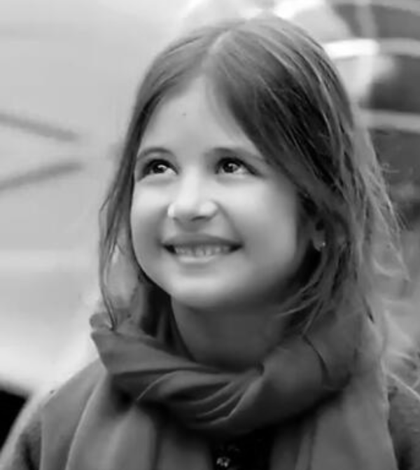
4.1.6 示例 原图:
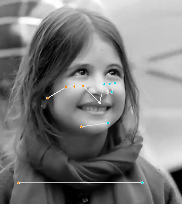
检测后:
注意为了显示自拍的效果,我将图片进行了水平翻转。
4.2 ORL 数据集 因为本次的姿态估计模型我是直接调用已经训练好的模型,因此只需要将 ORL 数据集当作测试集进行预测即可。
4.2.1 数据读取与处理 因为我们只需要数据集,因此不需要数据的标签与分割,同时因模型要求输入要是图片,则不需要对图片进行展平。此外,MediaPipe Pose 模型要求输入的图片是 RGB 类型,但是我们前面三个数据集的所有图片都是灰度图,则在检测前我们要将灰度图转成 RGB 图,同时不能改变图片的性质。怎么改呢?其实很简单:只需将该灰度图在通道维度拼接 3 次即可。此时,红色、绿色和蓝色的分量是相同的,因此图像仍然是 “灰度图”。
其实在技巧在前面使用 mtcnn 进行人脸检测时就使用过这个技巧,只是当时没有具体说明。我们在后续对 Yale 和 UMIST 数据集的姿态预测前会进行同样的处理,在此说明。
1
2
3
4
5
6
7
8
9
10
11
12
13
14
def Get_imgList (root ) : X = [] path_list = ['s' + str (i) for i in range (1 , 41 )] for idx, s in enumerate (path_list) : for i in range (1 , 11 ) : path = os.path.join(root, s, str (i) + '.pgm' ) img = Image.open (path) img = np.array(img) image = np.stack((img, img, img), axis=2 ) X.append(image) print (image.shape) return X
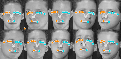
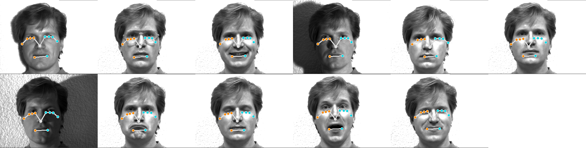
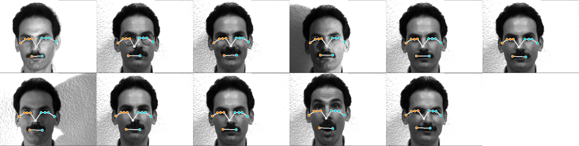
4.2.2 姿态估计 将第一和第二个人的姿态估计结果由如下代码进行拼接。
1
2
3
4
5
6
7
8
9
10
11
12
13
14
15
16
17
18
import cv2import numpy as npimg_path = ['ORL_Poses/pose_' + str (idx + 1 ) + '.png' for idx in range (20 )] img = [] for path in img_path : image = cv2.imread(path) img.append(image) img_1 = np.concatenate((img[0 : 5 ]), axis = 1 ) img_2 = np.concatenate((img[5 : 10 ]), axis = 1 ) img_3 = np.concatenate((img[10 : 15 ]), axis = 1 ) img_4 = np.concatenate((img[15 : 20 ]), axis = 1 ) img_5 = np.concatenate((img_1, img_2), axis = 0 ) img_6 = np.concatenate((img_3, img_4), axis = 0 ) cv2.imwrite('people_1.png' , img_5) cv2.imwrite('people_2.png' , img_6)
所得结果如下:
第一个人:
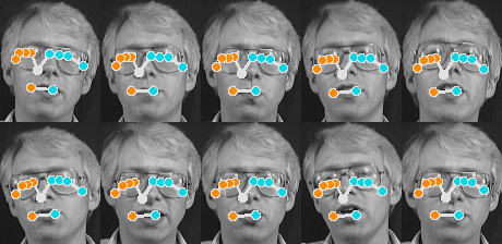
第二个人:
4.2.3 全部代码 1 2 3 4 5 6 7 8 9 10 11 12 13 14 15 16 17 18 19 20 21 22 23 24 25 26 27 28 29 30 31 32 33 34 35 36 37 38 39 40 41 42 43 44 45 46 47 48 49 50 51 52 53 54 55 import cv2import mediapipe as mpimport numpy as npimport osfrom PIL import Imagemp_drawing = mp.solutions.drawing_utils mp_drawing_styles = mp.solutions.drawing_styles mp_pose = mp.solutions.pose def Get_imgList (root ) : X = [] path_list = ['s' + str (i) for i in range (1 , 41 )] for idx, s in enumerate (path_list) : for i in range (1 , 11 ) : path = os.path.join(root, s, str (i) + '.pgm' ) img = Image.open (path) img = np.array(img) image = np.stack((img, img, img), axis=2 ) X.append(image) print (image.shape) return X def Pose (imgList ): with mp_pose.Pose( min_detection_confidence = 0.5 , min_tracking_confidence = 0.5 ) as pose: for idx, image in enumerate (imgList) : image.flags.writeable = False results = pose.process(image) image.flags.writeable = True mp_drawing.draw_landmarks( image, results.pose_landmarks, mp_pose.POSE_CONNECTIONS, landmark_drawing_spec = \ mp_drawing_styles.get_default_pose_landmarks_style()) cv2.imshow('MediaPipe Pose' , cv2.flip(image, 1 )) if idx < 20 : cv2.imwrite('ORL_Poses/pose_' + str (idx + 1 ) + '.png' , cv2.flip(image, 1 )) if cv2.waitKey(1 ) & 0xFF == 27 : break cv2.destroyAllWindows() imgList = Get_imgList('ORL' ) Pose(imgList)
4.3 Yale 数据集 对 Yale 数据集的姿态估计流程和 ORL 数据集一样,同时不用对 Yale 数据集进行人脸检测。对前面两个人的姿态估计效果如下:
第一个人:
第二个人:
全部代码:
1 2 3 4 5 6 7 8 9 10 11 12 13 14 15 16 17 18 19 20 21 22 23 24 25 26 27 28 29 30 31 32 33 34 35 36 37 38 39 40 41 42 43 44 45 46 47 48 49 50 51 52 53 54 55 56 57 58 59 60 61 62 63 64 65 66 67 68 69 70 71 72 73 74 75 76 77 78 79 80 import cv2import mediapipe as mpimport numpy as npimport osfrom PIL import Imagefrom skimage import iomp_drawing = mp.solutions.drawing_utils mp_drawing_styles = mp.solutions.drawing_styles mp_pose = mp.solutions.pose def Image_concatenate () : img_path = ['Yale_Poses/pose_' + str (idx + 1 ) + '.png' for idx in range (22 )] img = [] for idx, path in enumerate (img_path): image = cv2.imread(path) img.append(image) if idx == 10 or idx == 21 : noise = np.full(image.shape, 255 ).astype(np.uint8) print (noise.shape, noise.dtype) img.append(noise) img_1 = np.concatenate((img[0 : 6 ]), axis=1 ) img_2 = np.concatenate((img[6 : 12 ]), axis=1 ) img_3 = np.concatenate((img[12 : 18 ]), axis=1 ) img_4 = np.concatenate((img[18 : 24 ]), axis=1 ) img_5 = np.concatenate((img_1, img_2), axis=0 ) img_6 = np.concatenate((img_3, img_4), axis=0 ) cv2.imwrite('people_1.png' , img_5) cv2.imwrite('people_1.png' , img_6) def Get_imgList (root ) : Yale_path = [] X = [] for element in os.listdir(root): if element != 'Readme.txt' : Yale_path.append(os.path.join(root, element)) for path in Yale_path: img = io.imread(path, as_gray=True ) print (img.shape) image = np.stack((img, img, img), axis=2 ) X.append(image) return X def Pose (imgList ): with mp_pose.Pose( min_detection_confidence = 0.5 , min_tracking_confidence = 0.5 ) as pose: for idx, image in enumerate (imgList) : image.flags.writeable = False results = pose.process(image) image.flags.writeable = True mp_drawing.draw_landmarks( image, results.pose_landmarks, mp_pose.POSE_CONNECTIONS, landmark_drawing_spec = \ mp_drawing_styles.get_default_pose_landmarks_style()) cv2.imshow('MediaPipe Pose' , cv2.flip(image, 1 )) if idx < 22 : cv2.imwrite('Yale_Poses/pose_' + str (idx + 1 ) + '.png' , cv2.flip(image, 1 )) if cv2.waitKey(1 ) & 0xFF == 27 : break cv2.destroyAllWindows() imgList = Get_imgList('Yale' ) print (len (imgList))Pose(imgList)
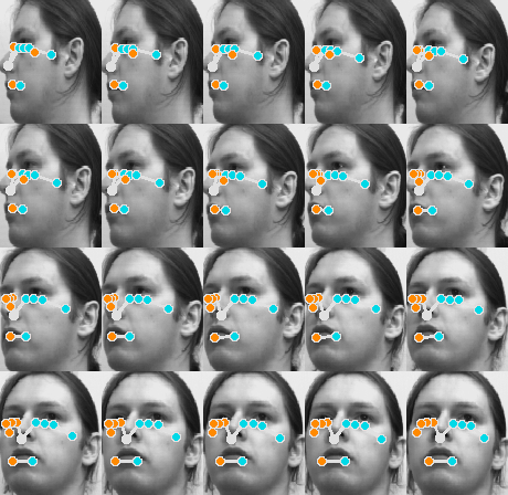
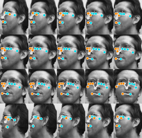
4.4 UMIST 数据集 因为 UMIST 中的图像是由人的侧面到正面进行拍摄的,因此我截取了第一和第二个人中间的二十张图片进行姿态估计的结果展示如下:
第一个人:
第二个人:
全部代码:
1 2 3 4 5 6 7 8 9 10 11 12 13 14 15 16 17 18 19 20 21 22 23 24 25 26 27 28 29 30 31 32 33 34 35 36 37 38 39 40 41 42 43 44 45 46 47 48 49 50 51 52 53 54 55 56 57 58 59 60 61 62 63 64 65 66 67 68 69 70 71 72 73 74 75 76 77 78 79 80 81 import cv2import mediapipe as mpimport numpy as npimport osfrom PIL import Imagemp_drawing = mp.solutions.drawing_utils mp_drawing_styles = mp.solutions.drawing_styles mp_pose = mp.solutions.pose def Image_concatenate () : img_path = ['UMIST_Poses/pose_' + str (idx + 1 ) + '.png' for idx in range (40 )] img = [] for idx, path in enumerate (img_path): image = cv2.imread(path) img.append(image) img_1 = np.concatenate((img[0 : 5 ]), axis=1 ) img_2 = np.concatenate((img[5 : 10 ]), axis=1 ) img_3 = np.concatenate((img[10 : 15 ]), axis=1 ) img_4 = np.concatenate((img[15 : 20 ]), axis=1 ) img_5 = np.concatenate((img[20 : 25 ]), axis=1 ) img_6 = np.concatenate((img[25 : 30 ]), axis=1 ) img_7 = np.concatenate((img[30 : 35 ]), axis=1 ) img_8 = np.concatenate((img[35 : 40 ]), axis=1 ) img_9 = np.concatenate((img_1, img_2, img_3, img_4), axis=0 ) img_10 = np.concatenate((img_5, img_6, img_7, img_8), axis=0 ) cv2.imwrite('people_5.png' , img_9) cv2.imwrite('people_6.png' , img_10) def Get_imgList (root ) : X = [] path_files = os.listdir(root) for idx, path_file in enumerate (path_files): path_images = os.listdir(os.path.join(root, path_file, 'face' )) for path_image in path_images: path = os.path.join(root, path_file, 'face' , path_image) img = Image.open (path) img = np.array(img) image = np.stack((img, img, img), axis=2 ) X.append(image) X = np.array(X) return X def Pose (imgList ): with mp_pose.Pose( min_detection_confidence = 0.5 , min_tracking_confidence = 0.5 ) as pose: for idx, image in enumerate (imgList) : image.flags.writeable = False results = pose.process(image) image.flags.writeable = True mp_drawing.draw_landmarks( image, results.pose_landmarks, mp_pose.POSE_CONNECTIONS, landmark_drawing_spec = \ mp_drawing_styles.get_default_pose_landmarks_style()) cv2.imshow('MediaPipe Pose' , cv2.flip(image, 1 )) if 10 <= idx < 30 : cv2.imwrite('UMIST_Poses/pose_' + str (idx + 1 - 10 ) + '.png' , cv2.flip(image, 1 )) if 48 <= idx < 68 : cv2.imwrite('UMIST_Poses/pose_' + str (idx + 1 - 28 ) + '.png' , cv2.flip(image, 1 )) if cv2.waitKey(1 ) & 0xFF == 27 : break cv2.destroyAllWindows() imgList = Get_imgList('UMIST' ) print (len (imgList))Pose(imgList)
4.5 结果分析 经过对三个数据集的中人的姿态估计,我们能够得到人脸关键部位点的位置,如左右眼角,左右嘴角,鼻子等,而根据这些关键特征点的分布我们可以对该人的形态或者神态进行进一步的预测。比如说,当眼睛那一排特征点的分布是水平的,说明这个人正处于一种较为平和、中立的状态,如果分布波动很大,则说明这个人此时正处于一种较为亢奋的状态,表现出愤怒、开心等表情;当特征点之间的距离很近,则对于摄像机而言这个人表现为侧脸;再者,当两个嘴角点之间的距离较大,即这个人的的嘴巴张的很大,我们可以觉得这个人是在开心大笑……等等。
综上,姿态分析对于视觉领域来说十分重要,我们可以利用姿态进行运动追踪、表情分析、医学诊断等等。
5 基于 KNN 的人脸识别 前面我们通过构建 PCA 降维算法分别对 ORL、Yale 和 UMIST 三种不同的数据集进行了人脸识别,且识别精度分别在 0.95、0.93 和 0.88。而在下面中,我使用了另一种传统机器学习算法——KNN 再次对上述三种数据集进行人脸识别。
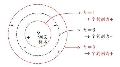
5.1 KNN KNN (K-Nearest Neighbor,K邻近算法)的基本思想是:给定一个训练数据集,对新输入的样本,在训练数据集中找到与该样本最邻近的 k 个实例(也就是所谓的 k 个邻居),这 k 个实例中的多数属于某个类别,就把输入样本划分到该类别中。k 近邻算法通常又可以分为分类算法和回归算法:
分类算法中采用多数表决法,就是选择 k 个样本中出现最多的类别标记作为预测结果;
回归算法中采用平均法,将 k 个样本实际输出标记的平均值或加权平均值作为预测结果。
而人脸识别本质上也是一个多分类问题,因此可以使用 KNN 来进行人脸识别。
5.2 ORL 数据集 首先是数据的读取与处理,KNN 接受的数据输入与 PCA 算法是一样的,即二维矩阵 (m,n),m 为样本数,n 为特征向量,因此数据处理与前面完全一样。
1
2
3
4
5
6
7
8
9
10
11
12
13
14
15
16
def Data_Processing (root ) : X = [] y = [] path_list = ['s' + str (i) for i in range (1 , 41 )] for idx, s in enumerate (path_list) : for i in range (1 , 11 ) : path = os.path.join(root, s, str (i) + '.pgm' ) img = Image.open (path) img = np.array(img).ravel() X.append(img) y.extend([idx] * 10 ) X = np.array(X) y = np.array(y) return X, y
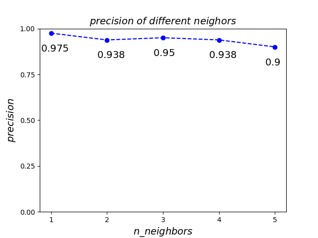
对于数据分组,我使用了 sklearn 库中的 train_test_split 函数,将数据划分成 2 : 8 ,其中训练集为 8,测试集为 2,同时将数据打乱。我还探究了不同 k 值对模型性能的影响。
1
2
3
4
5
6
7
8
9
10
11
12
13
14
15
16
17
18
19
20
21
22
23
24
25
26
27
28
29
30
def Draw_precision (scores ) : plt.plot(range (1 , 6 ), scores, 'o--' , color='blue' ) plt.xlabel('$n\_neighbors$' , fontsize=14 ) plt.ylabel('$precision$' , fontsize=14 ) for x, y in zip (range (1 , 6 ), scores): plt.text(x - 0.18 , y - 0.1 , f'${y} $' , fontsize=14 ) plt.title(f'$precision\ of\ different\ neighors$' , fontsize=14 ) plt.xticks(np.arange(1 , 6 )) plt.yticks(np.linspace(0 , 1 , 5 )) plt.show() plt.savefig('KNN_ORL_Database.png' ) if __name__ == '__main__' : X, y = Data_Processing('ORL' ) X_train, X_test, y_train, y_test = train_test_split(X, y, test_size=0.2 , \ train_size=0.8 , shuffle=True , random_state=42 ) scores = [] for n in range (1 , 6 ): knn = KNeighborsClassifier(n_neighbors=n) knn.fit(X_train, y_train) pred = knn.predict(X_test) score = round (knn.score(X_test, y_test), 3 ) scores.append(score) Draw_precision(scores)
所得结果如下:
如上图所示,k 等于 1 时人脸识别的效果最好,识别正确率达到 0.975,比 PCA 算法的 0.95 要高。
5.3 Yale 数据集 同理,参考 3.2.1 数据读取和数据处理
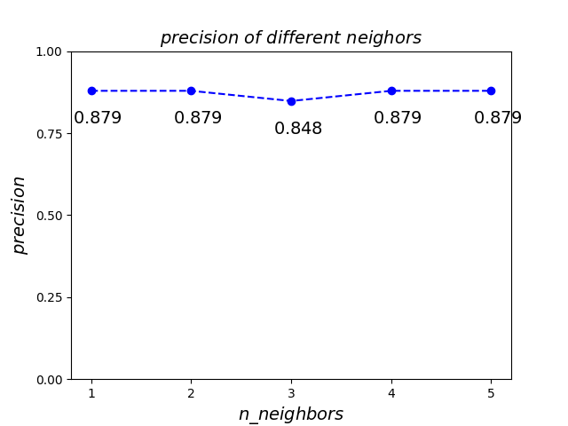
如上图所示,使用 KNN 对 Yale 进行识别的效果很不好,不同的 k 值中最高的识别正确率也只有 0.879。原因可能是数据过少,因为在训练之前进行了人脸检测并且裁剪。因此,我采取了下面的数据处理方式,即不进行人脸检测和裁剪等操作。
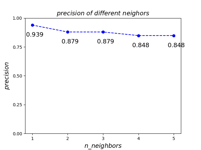
1
2
3
4
5
6
7
8
9
10
11
12
13
14
15
16
17
18
def Data_Processing (root ) : Yale_path = [] X = [] y = [] for element in os.listdir(root) : if element != 'Readme.txt' : Yale_path.append(os.path.join(root, element)) for path in Yale_path : image = io.imread(path, as_gray = True ) X.append(image.ravel()) label = int (os.path.split(path)[-1 ].split('.' )[0 ].replace("subject" , "" )) - 1 y.append(label) X = np.array(X) y = np.array(y) print (X.shape) return X, y
所得结果如下:
如上图所示,当 k 值为 1 时,模型的性能最好,即识别正确率达到 0.939,此结果与 PCA 算法相当。
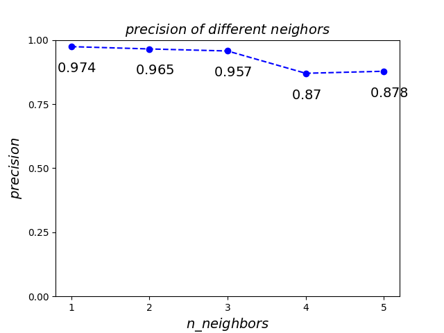
5.4 UMIST 数据集 UMIST 数据集的读取与处理参照 3.3.1 数据读取与数据处理
如上图所示,KNN 对于 UMIST 的鲁棒性非常强,识别性能特别好,在 k 等于 1、2 和 3 时的识别正确率有 0.974、0.965 和 0.957,远超 PCA 算法的 0.88 的正确率。
5.5 KNN 的优缺点 优点:
理论成熟,思想简单,既可以用来做分类又可以做回归;
可以用于非线性分类;
训练时间复杂度低,相比于 PCA,KNN 花费的时间很少;
和朴素贝叶斯之类的算法比,对数据没有假设,准确度高,对异常点不敏感;
由于 KNN 方法主要靠周围有限的邻近的样本,而不是靠判别类域的方法来确定所属的类别,因此对于类域的交叉或重叠较多的待分类样本集来说,KNN 方法较其他方法更为适合。
缺点:
计算量大,尤其是特征数非常多的时候;
样本不平衡的时候,对稀有类别的预测准确率低;
是惰性学习方法,基本上不学习,导致预测时速度比起逻辑回归之类的算法慢;
KNN 模型的可解释性不强。