1
2
3
4
5
6
7
8
9
10
11
12
13
14
15
16
17
18
19
20
21
22
23
24
25
26
27
28
29
30
31
32
33
34
35
36
37
38
39
40
41
42
43
44
45
46
47
48
49
50
51
52
53
54
55
56
57
58
59
60
61
62
63
64
65
66
67
68
69
70
71
72
73
74
75
76
77
78
79
80
81
82
83
84
85
86
87
88
89
90
91
92
93
94
95
96
97
98
99
100
101
102
103
104
105
106
107
108
109
110
111
112
113
114
115
116
117
118
119
120
121
122
123
124
125
126
127
128
129
130
| import matplotlib.pyplot as plt
import numpy as np
from scipy import optimize
import scipy.io as scio
%matplotlib
plt.rcParams["font.sans-serif"] = ["Simhei"]
plt.rcParams["axes.unicode_minus"] = False
data = scio.loadmat('2 data_preprocess_practice.mat')
yy3 = data["yy3"]
x = np.arange(0, 20001, 1)
def Noise_reduction(data_col) :
lst = []
i = 0
while i + 12 < 20001 :
lst1 = data_col[i : i + 12]
mean = np.mean(lst1)
std = np.std(lst1)
for value in lst1 :
if (value - mean) >= -3 * std and (value - mean) <= 3 * std :
lst.append(value)
i += 12
lst1 = []
return lst
def Average_sliding_denoising(arr, window_size) :
New_arr = arr[ : ]
window_size = (window_size - 1) // 2
for step in range(window_size) :
arr.insert(step, sum(arr[ : window_size]) / window_size)
arr.insert(len(arr) - step, sum(arr[len(arr) - window_size : len(arr)]) / window_size)
for i in range(window_size, len(arr) - window_size) :
New_arr[i - window_size] = (sum(arr[i - window_size : i + window_size + 1])) / (2 * window_size + 1)
return New_arr
def Exponential_sliding_denoising(arr, weight = 0.01) :
for i in range(1, len(arr)) :
arr[i] = weight * arr[i] + (1 - weight) * arr[i - 1]
return arr
def create_x(size, rank):
x = []
for i in range(2 * size + 1):
m = i - size
row = [m ** j for j in range(rank)]
x.append(row)
x = np.mat(x)
return x
def Savgol_Denosing(arr, window_size, rank) :
New_arr = arr[ : ]
m = (window_size - 1) // 2
for step in range(m) :
arr.insert(step, arr[0])
arr.insert(len(arr) - step, arr[len(arr) - 1])
X = create_x(m, rank)
B = (X * (X.T * X).I) * X.T
A0 = B[m].T
narr = []
for i in range(len(New_arr)):
y = [arr[i + j] for j in range(window_size)]
y1 = np.mat(y) * A0
y1 = float(y1)
narr.append(y1)
return narr
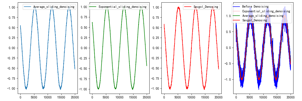
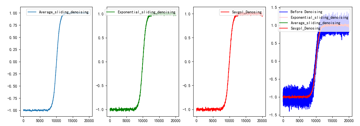
def Mapping(lst, arr, arr1, arr2) :
x = np.array(list(range(0, len(arr), 1)))
fig = plt.figure(figsize=(15, 5))
fig.set(alpha = 0.2)
plt.subplot2grid((1,4), (0, 0))
plt.plot(x, arr, label = 'Average_sliding_denoising')
plt.legend(loc = 1)
plt.subplot2grid((1, 4), (0, 1))
plt.plot(x, arr1, 'g-', label = 'Exponential_sliding_denoising')
plt.legend(loc = 1)
plt.subplot2grid((1, 4), (0, 2))
plt.plot(x, arr2, 'r-', label = 'Savgol_Denosing')
plt.legend(loc = 1)
plt.subplot2grid((1, 4), (0, 3))
plt.plot(x, lst, 'b-', x, arr, 'pink', x, arr1, 'g', x, arr2, 'r')
plt.legend(['Before Denoising', 'Exponential_sliding_denoising', 'Average_sliding_denoising', 'Savgol_Denosing'], loc = 1)
plt.show()
def Polynomial_fitting(lst) :
x1 = np.arange(0, len(lst), 1).astype(float)
z1 = np.polyfit(x1, lst, 11)
x_points = np.linspace(0, 19973, 19973)
y_point = np.polyval(z1, x_points)
fig1 = plt.figure()
plt.plot(x1, lst, x_points, y_point, 'r')
plt.legend(['Before fitting', 'After fitting'], loc = 1)
plt.show()
data_col1 = []
data_col2 = []
for line in yy3 :
data_col1.append(line[0])
data_col2.append(line[1])
data_col1 = np.array(data_col1)
data_col2 = np.array(data_col2)
lst1 = Noise_reduction(data_col1)
lst1_A = Average_sliding_denoising(Noise_reduction(data_col1), 61)
lst1_E = Exponential_sliding_denoising(Noise_reduction(data_col1))
lst1_S = Savgol_Denosing(Noise_reduction(data_col1), 59, 2)
Mapping(lst1, lst1_A, lst1_E, lst1_S)
Polynomial_fitting1(lst1_A)
|